Adding some level

 From previous code

Fractal Tree using Python with Turtle Module

Here is "minus one" nearly symmetrical fractal tree

import turtle
import numpy

#buat pola di sini
#kura-kura menghadap ke atas
turtle.shape("turtle")
turtle.left(90)


lv  = 7
l   = 100
s   = 17

turtle.penup()
turtle.backward(l)
turtle.pendown()
turtle.forward(l)


def maju(l,level):
    l           = 3./4.*l
    turtle.left(s)
    turtle.forward(l)
    if level<lv:
        level   +=1
        maju(l,level)
    
    turtle.backward(l)
    turtle.right(2*s)
    turtle.forward(l)
    if level<lv:
        maju(l,level)
    turtle.backward(l)
    turtle.left(s)
    level       -=1

maju(l,2)


#agar gambar tak langsung hilang
turtle.exitonclick()



 

.

if we want symmetrical result, just move 

level +=1 

syntax

to the place before first if

Some Mistake Often Provide Beautiful Result.

 :)

 Planned to coding tree branch of tree, fractal mode, using turtle module on python. Has some trouble on backward rule. It become flower, by definition, it's still tree, :)

import turtle

#buat pola di sini
#kura-kura menghadap ke atas
turtle.shape("turtle")
turtle.left(90)

s   = 37

lv  = 7

l   = 100
turtle.forward(l)

def mundur(l,level):
    l   = 4./3.*l
    turtle.backward(l)
    turtle.right(3*s)
    maju(l,level)

def maju(l,level):
    l   = 3./4.*l
    turtle.left(s)
    turtle.forward(l)
    level   +=1
    if level<=lv:
        maju(l,level)
    else:
        mundur(l,level)

maju(l,2)


#agar gambar tak langsung hilang
turtle.exitonclick()



 

.

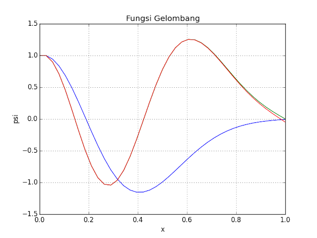
Even Wave Equation on Infinite-depth Potential Well (with Some Variation Potential in Between) using Shooting Method,

It's from previous code, I use it to simulate even function.

from pylab import *

figure(3)
n   = 39
psi0= zeros(n) #
psi = psi0     # 
x   = linspace(0,1,n)
V   = zeros(n)
#V   = 39*pow(x,2)

for i in arange(n):
    if i<n/2.:
        V[i]    = 73.
    else:
        V[i]    = 0.       

psi0[0] = 1.
psi0[1] = psi0[0] #for odd function, use another value, 

                  #but psi0[0] must be zero

t   = 0
dx  = 1./n
E   = 1.
dE  = .1
err = .05
while t< 771:
    #k   = 2*dx*dx*(E-V)
    for i in range (1,n-1):
        k   = 2*dx*dx*(E-V[i])
        psi[i+1]  = 2*psi0[i]-psi0[i-1]-k*psi0[i]
    psi0    = psi
    if abs(psi[n-1])<err:
        print E
        plot(x,psi)
    t   += 1
    E   += dE

xlabel('x')
ylabel('psi')
title('Fungsi Gelombang')
grid(True)
savefig("shooting.png")

figure(2)
plot(x,V)

xlabel('x')
ylabel('V')
title('Potensial')
grid(True)

show()

.
Here's some result with different potential V

Energy Quantization on Potential Well; Shooting Method, :) .

 Using Pylab module

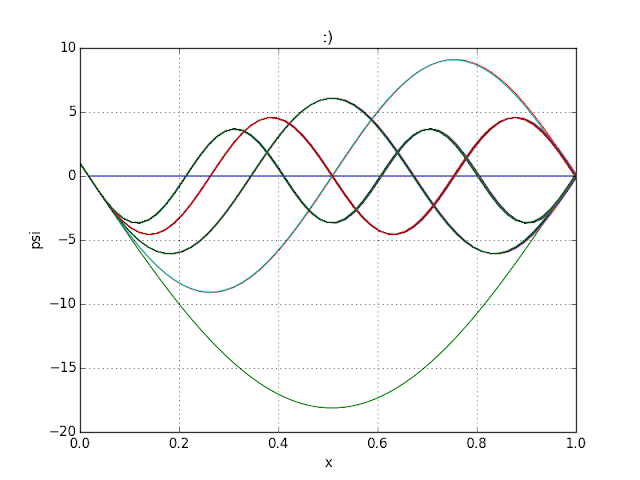
 Unlike the code before, only chosen energy with psi=0 on both end is plotted.

from pylab import *

n   = 59
psi0= zeros(n)
psi = psi0
x   = linspace(0,1,n)

psi0[0]  = 1.

plot(x,psi)

t   = 0
dx  = 1./16.
E   = 0.
dE  = .2
V   = 0.
while t< 1337:
    t   += 1
    E   += .01
    k   = 2*dx*dx*(E-V)
    for i in range (1,n-1):
        psi[i+1]  = 2*psi0[i]-psi0[i-1]-k*psi0[i]
    
    #psi[2:]   = 2*psi0[1:-1]-psi0[:-2]-k*psi0[1:-1]
    psi0    = psi
    #print psi[n-1]
    if abs(psi[n-1])<=dE:
        #pass
        print E
        plot(x,psi)


xlabel('x')
ylabel('psi')
title(':)')
grid(True)
savefig("els.png")
show()

.

Shooting Method on Potential Well

It's the base code I wrote using Python, still need improvement to get energy level or even what energy allowed in the system.

from pylab import *

n   = 19
psi0= zeros(n)
psi = psi0
x   = linspace(0,1,n)

psi0[0]  = 1.

plot(x,psi)

t   = 0
dx  = 1./8.
E   = .1
V   = 0.
while t< 27:
    t   += 1
    E   += .2
    k   = 2*dx*dx*(E-V)
    for i in range (1,n-1):
        psi[i+1]  = 2*psi0[i]-psi0[i-1]-k*psi0[i]
    
    psi0    = psi

    plot(x,psi)


xlabel('x')
ylabel('psi')
title(':)')
grid(True)
savefig("els.png")
show()

.

DLA Cluster in Python

 It's using random parameter, so if it'll show the different result every time it's executed.

"""
Cluster
"""
import numpy as np                          #untuk operasi array
import matplotlib.pyplot as plt             #untuk gambar grafik
import matplotlib.animation as animation    #untuk menggerakkan grafik

fig, ax = plt.subplots()

plt.ylim(0,40)
plt.xlim(0,40)
#variabel
n   = 39
x0   = 19
y0   = 19
a   = np.zeros((n,n))
a[x0,y0]  = 1
#print a
rx  = []    
ry  = []

#membuat garis/kurva dengan sumbu-x adalah x, sumbu-y adalah y
line, = ax.plot(x0, y0, 'o')

x0  = np.random.randint(n)
y0  = np.random.randint(n)
x   = x0
y   = y0

def animate(i):
    global line
    global x0,y0,rx,ry,n
          
    #menentukan seed baru
    x   = x0 + np.random.randint(-1,2)
    y   = y0 + np.random.randint(-1,2)
    
    #print 'x = ', x, ' y = ', y
    #apakah keluar batas?
    #apakah menyentuh cluster utama? 
    if (x>(n-2)) or (y>(n-2)) or (x<1) or (y<1) or\
            (a[x,y-1] + a[x,y] + a[x,y+1] + a[x-1,y-1] + a[x-1,y] + a[x-1,y+1] +\
            a[x+1,y-1] + a[x+1,y] + a[x+1,y+1]) >= 1:
        #renew()
        #update subcluster menjadi bagian dari cluster (0 ke 1)
        a[x,y]  = 1
        for i in np.arange(len(rx)):
            a[rx[i],ry[i]] = 1
        #print a
        ok  = 0
        while ok==0:
            x   = np.random.randint(n)
            y   = np.random.randint(n)
            #cek
            if (a[x,y]==0) and (x>1) and (y>1) and (x<(n-2))and (y<(n-2)):
                ok  = 1
        ok  = 0
        #kosongkan 
        #print 'rx', rx
        rx  = []
        ry  = []
        #print 'rx',rx
        
    #print 'xnew = ', x, ' y = ', y

    #setelah mendapatkan seed baru, rekam titiknya
    rx.append(x)
    ry.append(y)
    x0  = x
    y0  = y
    
    line, = ax.plot(x,y,'o')
    return line,

ani = animation.FuncAnimation(fig, animate, frames=777, interval=100, blit=False)
ani.save('clusterDLA.mp4',bitrate=1024)
#plt.show()

.

3D (Polar/Cylindrical Coordinate) Animation of 2D Diffusion Equation using Python, Scipy, and Matplotlib

 Yup, that same code but in polar coordinate.

 I use nabla operator for cylindrical coordinate but ditch the z component.

 So, what's the z-axis for? It's represent the u value, in this case, temperature, as function of r and phi (I know I should use rho, but, ...)

import scipy as sp

from mpl_toolkits.mplot3d import Axes3D
from matplotlib import cm
from matplotlib.ticker import LinearLocator, FormatStrFormatter
import matplotlib.pyplot as plt

import mpl_toolkits.mplot3d.axes3d as p3
import matplotlib.animation as animation

#dr  = .1
#dp  = .1
#nr      = int(1/dr)
#np      = int(2*sp.pi/dp)


nr  = 10
np  = 10

r       = sp.linspace(0.,1.,nr)
p       = sp.linspace(0.,2*sp.pi,np)

dr  = r[1]-r[0]
dp  = p[1]-p[0]

a   = .5

tmax    = 100
t       = 0.


dr2     = dr**2
dp2     = dp**2

dt      = dr2 * dp2 / (2 * a * (dr2 + dp2) )
dt      /=10.
print 'dr = ',dr 
print 'dp = ',dp 
print 'dt = ',dt



ut      = sp.zeros([nr,np])
u0      = sp.zeros([nr,np])

ur      = sp.zeros([nr,np])
ur2     = sp.zeros([nr,np])


#initial

for i in range(nr):
    for j in range(np):
        if ((i>4)&(i<6)):
            u0[i,j] = 1.
#print u0

def hitung_ut(ut,u0):
    for i in sp.arange (len(r)):
        if r[i]!= 0.:
            ur[i,:]     = u0[i,:]/r[i]
            ur2[i,:]     = u0[i,:]/(r[i]**2)
    ut[1:-1, 1:-1]  = u0[1:-1, 1:-1] + a*dt*(
            (ur[1:-1, 1:-1] - ur[:-2, 1:-1])/dr+
            (u0[2:, 1:-1] - 2*u0[1:-1, 1:-1] + u0[:-2,1:-1])/dr2+
            (ur2[1:-1, 2:] - 2*ur2[1:-1, 1:-1] + ur2[1:-1, :-2])/dp2)
    #calculate the edge
    ut[1:-1, 0]  = u0[1:-1, 0] + a*dt*(
            (ur[1:-1, 0] - ur[:-2, 0])/dr+
            (u0[2:, 0] - 2*u0[1:-1, 0] + u0[:-2, 0])/dr2+
            (ur2[1:-1, 1] - 2*ur2[1:-1, 0] + ur2[1:-1, np-1])/dp2)
    ut[1:-1, np-1]  = u0[1:-1, np-1] + a*dt*(
            (ur[1:-1, np-1] - ur[:-2, np-1])/dr+
            (u0[2:, np-1] - 2*u0[1:-1, np-1] + u0[:-2,np-1])/dr2+
            (ur2[1:-1, 0] - 2*ur2[1:-1, np-1] + ur2[1:-1, np-2])/dp2)


#hitung_ut(ut,u0)
#print ut

def data_gen(framenumber, Z ,surf):
    global ut
    global u0
    global t
    hitung_ut(ut,u0)
    u0[:] = ut[:]
    Z = u0
    t += 1
    print t
    
    ax.clear()
    plotset()
    surf = ax.plot_surface(X, Y, Z, rstride=1, cstride=1, cmap=cm.coolwarm,
                       linewidth=0, antialiased=False, alpha=0.7)
    return surf,


fig = plt.figure()
#ax = fig.gca(projection='3d')
ax = fig.add_subplot(111, projection='3d')

P,R = sp.meshgrid(p,r)

X,Y = R*sp.cos(P),R*sp.sin(P) 

Z = u0
print len(R), len(P)



def plotset():
    ax.set_xlim3d(-1., 1.)
    ax.set_ylim3d(-1., 1.)
    ax.set_zlim3d(-1.,1.)
    ax.set_autoscalez_on(False)
    ax.zaxis.set_major_locator(LinearLocator(10))
    ax.zaxis.set_major_formatter(FormatStrFormatter('%.02f'))
    cset = ax.contour(X, Y, Z, zdir='x', offset=-1. , cmap=cm.coolwarm)
    cset = ax.contour(X, Y, Z, zdir='y', offset=1. , cmap=cm.coolwarm)
    cset = ax.contour(X, Y, Z, zdir='z', offset=-1., cmap=cm.coolwarm)

plotset()
surf = ax.plot_surface(X, Y, Z, rstride=1, cstride=1, cmap=cm.coolwarm,
                       linewidth=0, antialiased=False, alpha=0.7)

fig.colorbar(surf, shrink=0.5, aspect=5)

ani = animation.FuncAnimation(fig, data_gen, fargs=(Z, surf),frames=4096, interval=4, blit=False)
#ani.save('2dDiffusionfRadialf1024b512.mp4', bitrate=1024)

plt.show()    

.

100x100 size

The Wrong Code Will often Provide Beautiful Result, :)

 It means to compute 2d diffusion equation just like previous post in polar/cylindrical coordinate, and all went to wrong direction, :)

 Still trying to understand matplotlib mplot3d behavior

import scipy as sp

from mpl_toolkits.mplot3d import Axes3D
from matplotlib import cm
from matplotlib.ticker import LinearLocator, FormatStrFormatter
import matplotlib.pyplot as plt

import mpl_toolkits.mplot3d.axes3d as p3
import matplotlib.animation as animation

#dr  = .1
#dp  = .1
#nr      = int(1/dr)
#np      = int(2*sp.pi/dp)

nr  = 10
np  = 10

dr  = 1./nr
dp  = 2*sp.pi/np

a   = .5

tmax    = 100
t       = 0.


dr2     = dr**2
dp2     = dp**2

dt      = dr2 * dp2 / (2 * a * (dr2 + dp2) )
dt      /=10.
print dt



ut      = sp.zeros([nr,np])
u0      = sp.zeros([nr,np])

ur      = sp.zeros([nr,np])
ur2     = sp.zeros([nr,np])

r       = sp.arange(0.,1.,dr)
p       = sp.arange(0.,2*sp.pi,dp)

#initial

for i in range(nr):
    for j in range(np):
        if ( (i>(2*nr/5.)) & (i<(3.*nr/3.)) ):
            u0[i,j] = 1.
#print u0

def hitung_ut(ut,u0):
    for i in sp.arange (len(r)):
        if r[i]!= 0.:
            ur[i,:]     = u0[i,:]/r[i]
            ur2[i,:]     = u0[i,:]/(r[i]**2)
    ut[1:-1, 1:-1]  = u0[1:-1, 1:-1] + a*dt*(
            (ur[1:-1, 1:-1] - ur[:-2, 1:-1])/dr+
            (u0[2:, 1:-1] - 2*u0[1:-1, 1:-1] + u0[:-2,1:-1])/dr2+
            (ur2[1:-1, 2:] - 2*ur2[1:-1, 1:-1] + ur2[1:-1, :-2])/dp2)


#hitung_ut(ut,u0)
#print ut


def data_gen(framenumber, Z ,surf):
    global ut
    global u0
    hitung_ut(ut,u0)
    u0[:] = ut[:]
    Z = u0
    
    ax.clear()
    plotset()
    surf = ax.plot_surface(X, Y, Z, rstride=1, cstride=1, cmap=cm.coolwarm,
                       linewidth=0, antialiased=False, alpha=0.7)
    return surf,


fig = plt.figure()
#ax = fig.gca(projection='3d')
ax = fig.add_subplot(111, projection='3d')

R = sp.arange(0,1,dr)
P = sp.arange(0,2*sp.pi,dp)
R,P = sp.meshgrid(R,P)

X,Y = R*sp.cos(P),R*sp.sin(P) 

Z = u0
print len(R), len(P)



def plotset():
    ax.set_xlim3d(-1., 1.)
    ax.set_ylim3d(-1., 1.)
    ax.set_zlim3d(-1.,1.)
    ax.set_autoscalez_on(False)
    ax.zaxis.set_major_locator(LinearLocator(10))
    ax.zaxis.set_major_formatter(FormatStrFormatter('%.02f'))
    cset = ax.contour(X, Y, Z, zdir='x', offset=0. , cmap=cm.coolwarm)
    cset = ax.contour(X, Y, Z, zdir='y', offset=1. , cmap=cm.coolwarm)
    cset = ax.contour(X, Y, Z, zdir='z', offset=-1., cmap=cm.coolwarm)

plotset()
surf = ax.plot_surface(X, Y, Z, rstride=1, cstride=1, cmap=cm.coolwarm,
                       linewidth=0, antialiased=False, alpha=0.7)

fig.colorbar(surf, shrink=0.5, aspect=5)

ani = animation.FuncAnimation(fig, data_gen, fargs=(Z, surf),frames=500, interval=30, blit=False)
#ani.save('2dDiffusionf500b512.mp4', bitrate=512)

plt.show()    

.

3D Animation of 2D Diffusion Equation using Python, Scipy, and Matplotlib

 I wrote the code on OS X El Capitan, use a small mesh-grid.  Basically it's same code like the previous post.

 I use surface plot mode for the graphic output and animate it.

 Because my Macbook Air is suffered from running laborious code, I save the animation on my Linux environment, 1024 bitrate, 1000 frames.

story

import scipy as sp
import time
from mpl_toolkits.mplot3d import Axes3D
from matplotlib import cm
from matplotlib.ticker import LinearLocator, FormatStrFormatter
import matplotlib.pyplot as plt

import mpl_toolkits.mplot3d.axes3d as p3
import matplotlib.animation as animation



dx=0.01        
dy=0.01     
a=0.5          
timesteps=500  
t=0.

nx = int(1/dx)
ny = int(1/dy)


dx2=dx**2 
dy2=dy**2 

dt = dx2*dy2/( 2*a*(dx2+dy2) )

ui = sp.zeros([nx,ny])
u = sp.zeros([nx,ny])

for i in range(nx):
 for j in range(ny):
  if ( ( (i*dx-0.5)**2+(j*dy-0.5)**2 <= 0.1)
   & ((i*dx-0.5)**2+(j*dy-0.5)**2>=.05) ):
    ui[i,j] = 1
def evolve_ts(u, ui):
 u[1:-1, 1:-1] = ui[1:-1, 1:-1] + a*dt*( 
                (ui[2:, 1:-1] - 2*ui[1:-1, 1:-1] + ui[:-2, 1:-1])/dx2 + 
                (ui[1:-1, 2:] - 2*ui[1:-1, 1:-1] + ui[1:-1, :-2])/dy2 )
        

def data_gen(framenumber, Z ,surf):
    global u
    global ui
    evolve_ts(u,ui)
    ui[:] = u[:]
    Z = ui
    
    ax.clear()
    plotset()
    surf = ax.plot_surface(X, Y, Z, rstride=1, cstride=1, cmap=cm.coolwarm,
                       linewidth=0, antialiased=False, alpha=0.7)
    return surf,


fig = plt.figure()
ax = fig.add_subplot(111, projection='3d')

X = sp.arange(0,1,dx)
Y = sp.arange(0,1,dy)
X,Y= sp.meshgrid(X,Y)

Z = ui 

def plotset():
    ax.set_xlim3d(0., 1.)
    ax.set_ylim3d(0., 1.)
    ax.set_zlim3d(-1.,1.)
    ax.set_autoscalez_on(False)
    ax.zaxis.set_major_locator(LinearLocator(10))
    ax.zaxis.set_major_formatter(FormatStrFormatter('%.02f'))
    cset = ax.contour(X, Y, Z, zdir='x', offset=0. , cmap=cm.coolwarm)
    cset = ax.contour(X, Y, Z, zdir='y', offset=1. , cmap=cm.coolwarm)
    cset = ax.contour(X, Y, Z, zdir='z', offset=-1., cmap=cm.coolwarm)

plotset()
surf = ax.plot_surface(X, Y, Z, rstride=1, cstride=1, cmap=cm.coolwarm,
                       linewidth=0, antialiased=False, alpha=0.7)


fig.colorbar(surf, shrink=0.5, aspect=5)

ani = animation.FuncAnimation(fig, data_gen, fargs=(Z, surf),frames=1000, interval=30, blit=False)
ani.save("2dDiffusion.mp4", bitrate=1024)

#plt.show()    

.

2D Diffusion Equation using Python, Scipy, and VPython

 I got it from here, but modify it here and there.

 I also add animation using vpython but can't find 3d or surface version, so I planned to go to matplotlib surface plot route, :)

 (update: here it is, :) )

#!/usr/bin/env python
"""
A program which uses an explicit finite difference
scheme to solve the diffusion equation with fixed
boundary values and a given initial value for the
density.

Two steps of the solution are stored: the current
solution, u, and the previous step, ui. At each time-
step, u is calculated from ui. u is moved to ui at the
end of each time-step to move forward in time.

http://www.timteatro.net/2010/10/29/performance-python-solving-the-2d-diffusion-equation-with-numpy/

he uses matplotlib

I use visual python

"""
import scipy as sp
import time
from visual import *
from visual.graph import *


graph1 = gdisplay(x=0, y=0, width=600, height=400, 
          title='x vs. T', xtitle='x', ytitle='T', 
          foreground=color.black, background=color.white)


# Declare some variables:

dx=0.01        # Interval size in x-direction.
dy=0.01        # Interval size in y-direction.
a=0.5          # Diffusion constant.
timesteps=500  # Number of time-steps to evolve system.
t=0.

nx = int(1/dx)
ny = int(1/dy)

dx2=dx**2 # To save CPU cycles, we'll compute Delta x^2
dy2=dy**2 # and Delta y^2 only once and store them.

# For stability, this is the largest interval possible
# for the size of the time-step:
dt = dx2*dy2/( 2*a*(dx2+dy2) )

# Start u and ui off as zero matrices:
ui = sp.zeros([nx,ny])
u = sp.zeros([nx,ny])

# Now, set the initial conditions (ui).
for i in range(nx):
 for j in range(ny):
  if ( ( (i*dx-0.5)**2+(j*dy-0.5)**2 <= 0.1)
   & ((i*dx-0.5)**2+(j*dy-0.5)**2>=.05) ):
    ui[i,j] = 1
'''
def evolve_ts(u, ui):
 global nx, ny
 """
 This function uses two plain Python loops to
 evaluate the derivatives in the Laplacian, and
 calculates u[i,j] based on ui[i,j].
 """
 for i in range(1,nx-1):
  for j in range(1,ny-1):
   uxx = ( ui[i+1,j] - 2*ui[i,j] + ui[i-1, j] )/dx2
   uyy = ( ui[i,j+1] - 2*ui[i,j] + ui[i, j-1] )/dy2
   u[i,j] = ui[i,j]+dt*a*(uxx+uyy)
'''
def evolve_ts(u, ui):
 """
 This function uses a numpy expression to
 evaluate the derivatives in the Laplacian, and
 calculates u[i,j] based on ui[i,j].
 """
 u[1:-1, 1:-1] = ui[1:-1, 1:-1] + a*dt*( 
                (ui[2:, 1:-1] - 2*ui[1:-1, 1:-1] + ui[:-2, 1:-1])/dx2 + 
                (ui[1:-1, 2:] - 2*ui[1:-1, 1:-1] + ui[1:-1, :-2])/dy2 )
        
# Now, start the time evolution calculation...
#tstart = time.time()

f1 = gcurve(color=color.blue)

while True:
    rate(60)
    #for m in range(1, timesteps+1):
    if t<timesteps:
        t+=dt
 evolve_ts(u, ui)
        ui[:] = u[:] # I add this line to update ui value (not present in original code)
 #print "Computing u for m =", m
    f1.gcurve.pos   =   []
    for i in arange(nx):
        f1.plot(pos=(i,u[nx/2,i]))
    
#tfinish = time.time()

#print "Done."
#print "Total time: ", tfinish-tstart, "s"
#print "Average time per time-step using numpy: ", ( tfinish - tstart )/timesteps, "s."

.

Numpy Slice Expression

 Suppossed we have two array a and b

 If we want to set b as finite difference result of a, we may tempted to do this

for i in range (9):
 b[i] = a[i+1]-a[i]

There's another (faster) way. The performance's close to the pure C, :)

b[:-1] = a[1:]-a[:-1]

What's that?

Numpy has slice form for array. If we have an array with length 10, the a[:] refers to all value in a.

a[1:] refers to a[1] to a[9] (without a[0])
a[3:] refers to a[3] to a[9]
a[:-1] refers to a[0] to a[8]
a[:-3] refers to a[0] to a[6]
a[1:-1] refers to a[1] to a[8]
...
and so on

Here's my tinkering with slice expression

>>> from numpy import *
>>> a = zeros(10)
>>> b = zeros(10)
>>> a[5]=1.
>>> a
array([ 0.,  0.,  0.,  0.,  0.,  1.,  0.,  0.,  0.,  0.])
>>> b
array([ 0.,  0.,  0.,  0.,  0.,  0.,  0.,  0.,  0.,  0.])
>>> a[6]=2.
>>> a
array([ 0.,  0.,  0.,  0.,  0.,  1.,  2.,  0.,  0.,  0.])
>>> b[:-1]=a[:-1]-a[1:]
>>> b
array([ 0.,  0.,  0.,  0., -1., -1.,  2.,  0.,  0.,  0.])
>>> b[:-1]=a[:-1]+a[1:]
>>> b
array([ 0.,  0.,  0.,  0.,  1.,  3.,  2.,  0.,  0.,  0.])
>>> 

I like Python, :)

Create CSV file using Delphi

 I used textfile variable to write to a file (or create it if it don't exist).

 CSV file? Just make sure that the name at assignfile  command had .csv extension, :)

 Of course we have to format the output to meet the CSV standart; separated by comma.

procedure TForm1.Button1Click(Sender: TObject);
var
    fileku:textfile;
    i,j,n:integer;
begin
  n:=10;
  assignfile(fileku,'data.csv');
  rewrite(fileku);
  writeln(fileku,'tadaa...');
  for i:=1 to n do begin
    for j:=1 to n do begin
      writeln(fileku,i,',',j,',','data',i,j);
    end;
  end;
  closefile(fileku);
end;

.

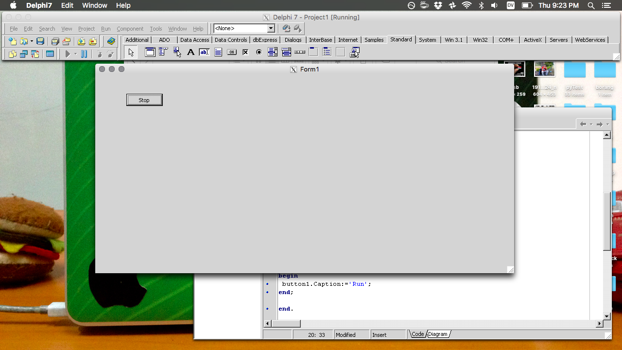
Delphi on OS X

 Here's the WineSkin version.

 I found it's way smoother than WineBottler version, ...., but hard to figure how to use it

 To install Delphi in OS X using WineSkin, we have to download and install Wineskin, of course, :)

• Open Wineskin Winery.app
• Make sure you have a Wrapper version and an Engine
• Select the Engine you want to use (I use WS9Wine1.7.52)
• Press the Create Wrapper button
• Enter in the name Delphi (or whatever you have in mind) for the wrapper and press OK
• When its done being created, click the button to view it in Finder in the finished window
• Close Wineskin Winery.app.
• Right click Delphi.app in Finder and select “Show Package Contents”
• Double click and run Wineskin.app.
• Now click on the Install Software button
• Select to choose a setup executable
• Navigate to the Delphi setup exe file you downloaded in step one
• Select the setup exe file and press the choose button
• At this point Delphi setup should begin, go through the Delphi setup like a normal install
• After the setup is done, back in Wineskin.app, it should pop up asking you to select the .exe file
• Choose the delphi32.exe file in the drop down list and press the Select Button
• Now press the Quit button to exit Wineskin.app
• Back in Finder, double click Delphi.app and start coding

 It has the same problem with WineBottler,  the toolbar tab's seem order by itself alphabetically, so the default toolbar tab is not ' standard ' tab but 'additional' one

code
unit Unit1;

interface

uses
  Windows, Messages, SysUtils, Variants, Classes, Graphics, Controls, Forms,
  Dialogs, StdCtrls;

type
  TForm1 = class(TForm)
    Button1: TButton;
    procedure Button1Click(Sender: TObject);
    procedure FormCreate(Sender: TObject);
  private
    { Private declarations }
  public
    { Public declarations }
  end;

var
  Form1: TForm1;
  jalan:boolean=false;

implementation

{$R *.dfm}

procedure TForm1.Button1Click(Sender: TObject);
begin
  jalan := not jalan;
  if jalan = true then button1.Caption:='Stop'
    else button1.Caption:='Run';

end;

procedure TForm1.FormCreate(Sender: TObject);
begin
 button1.Caption:='Run';
end;

end.

.

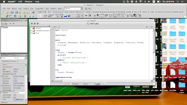
Delphi on OS X

 I use WineBottler to install Delphi 7 on my El Capitan.

 It's installed, it can run.

 The one that tickle me is the toolbar list is scrambled, it's sorted alphabetically, so additional toolbar is in the first and act as default toolbar.

code

SwishMax in Mac.

  :)

 Yeah, I use OS X El Capitan in My Macbook Air and use Wine Bottler to install it.

 Make sure that flash option is ticked in winetriks part